Mood tracking 2025
Introduction
2025 has been an important year for me. I reached several milestones, including publishing my first first-author academic paper, remarkably on my birthday, and successfully defending my prospectus, the final step before graduation. I also met new people, formed meaningful connections, and lost some along the way.
This marked my fourth year in the United States, and I realized that my mood fluctuated more throughout this year than at any other time in my life, more than the previous three years abroad, and even more than the over twenty years I spent in China. With gains and losses intertwined, the year felt like a roller coaster I did not choose to board. Occasionally, it paused, leaving me sitting alone, able to hear my own thoughts clearly.
Throughout 2025, I tracked my mood daily. Here, I chose to present these data in the way I have been trained during my PhD. If you find this interesting or would like to discuss anything, you are always welcome to reach out.
Daily mood dynamics across the calendar year
“Gray November, I’ve been down since July.”
— Evermore, Taylor Swift
As one of the greatest poets of our time, Taylor Swift captures how mood can vary with time—particularly across months. Fig. 1A presents a calendar view of my daily mood throughout 2025, with color representing mood intensity. Blue tones indicate depressive states, whereas green tones indicate happiness, as shown by the color bar below. Fig. 1B shows mood scores over months, providing a direct illustration of mood of the year. Three-day rolling averaged trend (Fig. 1C) shows three clear valleys in between other fine days.
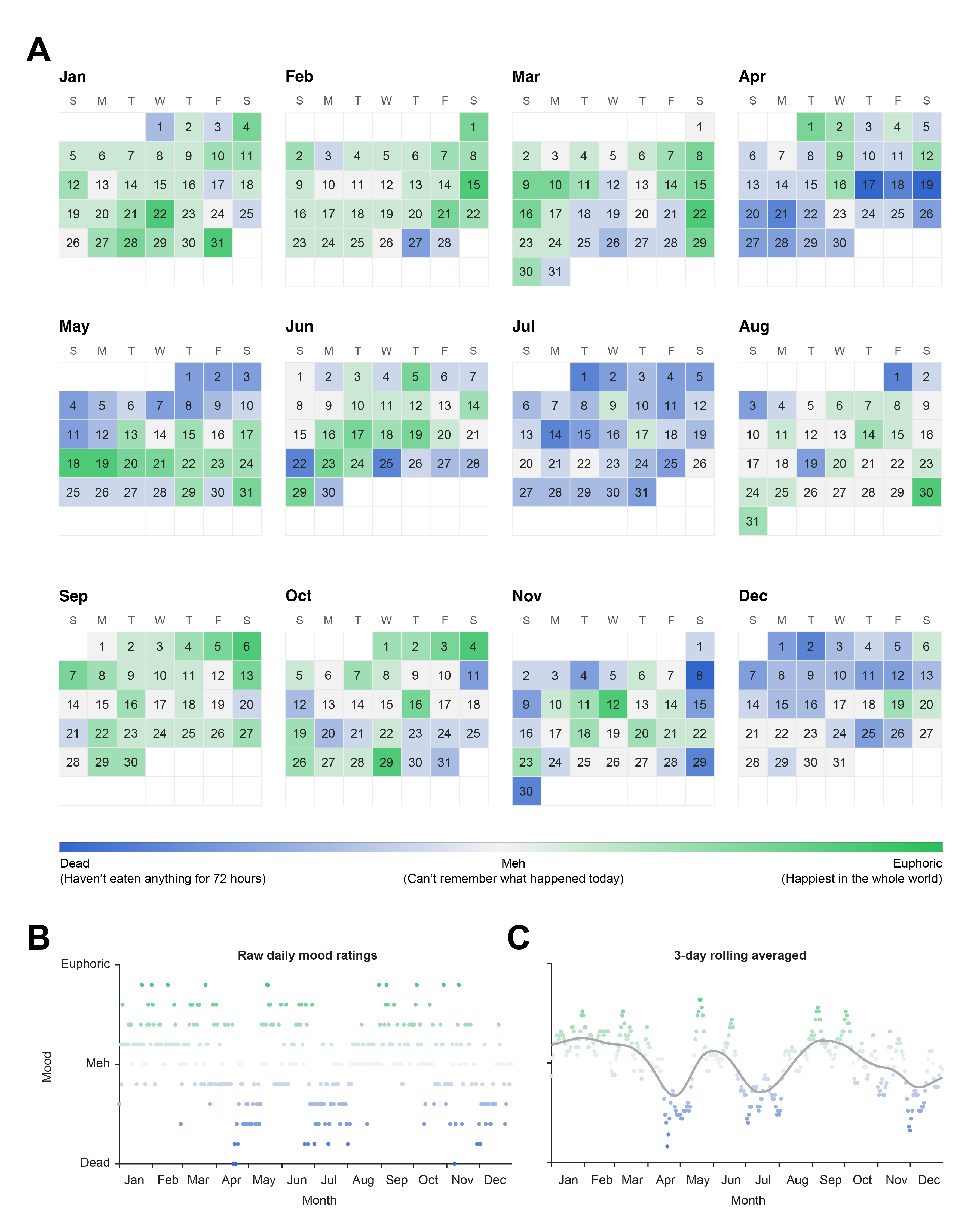
Figure 1. A. Calendar heatmap of daily mood scores throughout the year. Each cell represents one day, colored by mood value. B. Raw daily mood scores plotted over months. Each point represents one day. C. Three-day rolling average of daily mood, overlaid on low-frequency trends while preserving day-to-day variability.
Temporal structure of mood across months, days, seasons, and academic cycles
To further investigate the temporal structure of mood, I grouped daily scores by month (Fig. 2A). Mood was significantly lower in April compared to the previous month (t(353) = 4.576, p < 0.0001), as well as in July compared to June (t(353) = 4.734, p < 0.0001). However, it increased significantly in August (t(353) = 4.454, p = 0.001), suggesting a partial recovery during that period.
No significant differences were observed between October and November, or between November and December. This suggests that despite an overall depressive trend late in the year, occasional positive days temporarily elevated my mood—what felt like hope at the time, but in retrospect, proved transient.
Although no additional adjacent monthly comparisons reached significance (ts(353) ≤ 2.442, ps ≥ 0.154), the distributional analysis (Fig. 2B) revealed meaningful structure. April and May exhibited bimodal distributions, indicating alternating periods of happiness and sadness within the same month, whereas most other months showed unimodal distributions that gradually shifted left or right over time.
Further, there were no differences in mood across days of the week (Fig. 2C; qs(358) ≤ 2.145, ps ≥ 0.735). However, mood was significantly better in the fall than in the summer (Fig. 2D; t(361) = 3.056, p = 0.007).
Within the academic calendar, I was happier in the spring semester than during the break between spring and summer semesters (Fig. 2E; t(354) = 4.165, p = 0.0003), and mood was rescued during the summer break (t(354) = 3.263, p = 0.008).
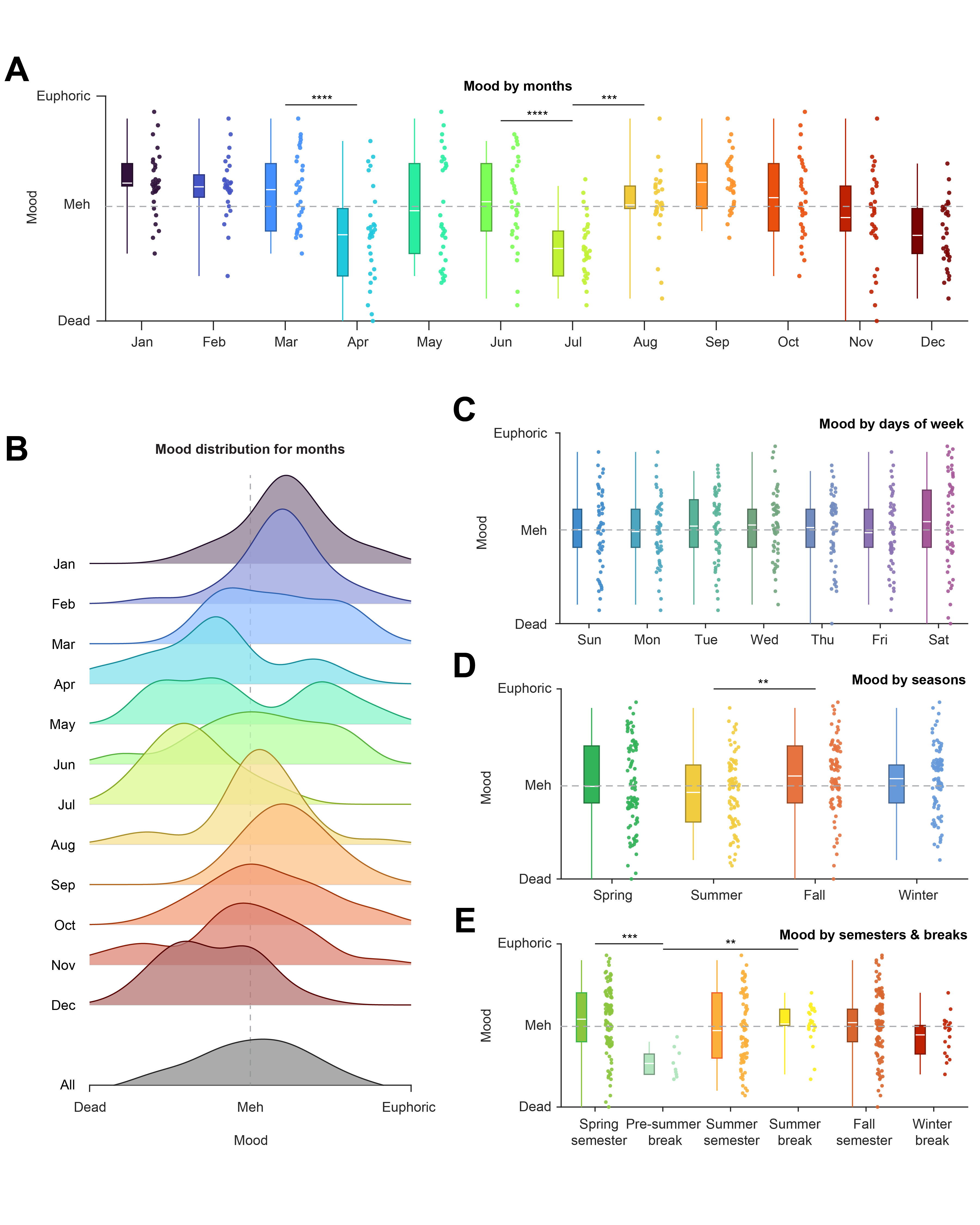
Figure 2. A. Distribution of daily mood scores across calendar months. Boxes indicate the interquartile range (25–75%), central white line denotes the mean, and whiskers span the full range. Individual daily observations are shown as individual points, jittered by a little for illustration purposes. Dashed line indicates the neutral mood baseline (“Meh”). B. Ridgeline density estimates of mood distributions for each month and for all months pooled. Curves represent kernel density estimates normalized to equal height. Dashed vertical line marks the neutral mood level. C. Mood distributions stratified by days of the week. Plot elements as in panel A. D. Mood distributions grouped by meteorological seasons. Seasons are defined by calendar months. Spring: March, April, and May. Summer: Jun, July, and August. Fall: September, October, and November. Winter: December, January, and February. E. Mood distributions across academic semesters and inter-semester breaks. Spring semester: 1/6 - 5/2. Pre-summer break: 5/3 - 5/11. Summer semester: 5/12 - 8/1. Summer break: 8/2 - 8/24. Fall semester: 8/25 - 12/12. Winter break: 12/13 - 12/31. ** P < 0.01, *** P < 0.001, **** P < 0.0001
Event-triggered mood dynamics following positive and negative experiences
To examine short-term mood dynamics, I identified joyful days (mood ≥ 7) and aligned mood trajectories from seven days before to seven days after each event (Fig. 3A). On average, mood was substantially lower the day before joyful events (4.92 → 7.45; Δ = +2.53), remained elevated the following day (7.45 → 5.84; Δ = −1.61), and returned toward neutral approximately five days later (score = 5.12).
Nearly two-thirds of joyful events involved talking to or spending quality time with people I like, followed by travel, engaging in sports, and general social events. I was also very happy when my first first-author paper was accepted and when I heard rumors that I could stay in New York City for one to two weeks to learn a new technique, though neither happiness lasted long (Fig. 3B).
In contrast, depressive events (mood ≤ 3) showed a different temporal profile (Fig. 3C). Mood declined sharply from the day before to the event day (4.76 → 2.22; Δ = −2.54) and recovered only partially the following day (2.22 → 3.64; Δ = +1.42). Even seven days later, mood had not returned to neutral levels (score = 4.59).
Overthinking accounted for approximately 70% of depressive events (Fig. 3D). As Taylor Swift writes in Evermore:
“I replay my footsteps on each stepping stone
Trying to find the one where I went wrong
Writing letters
Addressed to the fire”“I rewind the tape but all it does is pause
On the very moment all was lost
Sending signals
To be double crossed”— Evermore, Taylor Swift
This precisely captures my experience. Other contributors included last-minute plan cancellations and illness or injury.
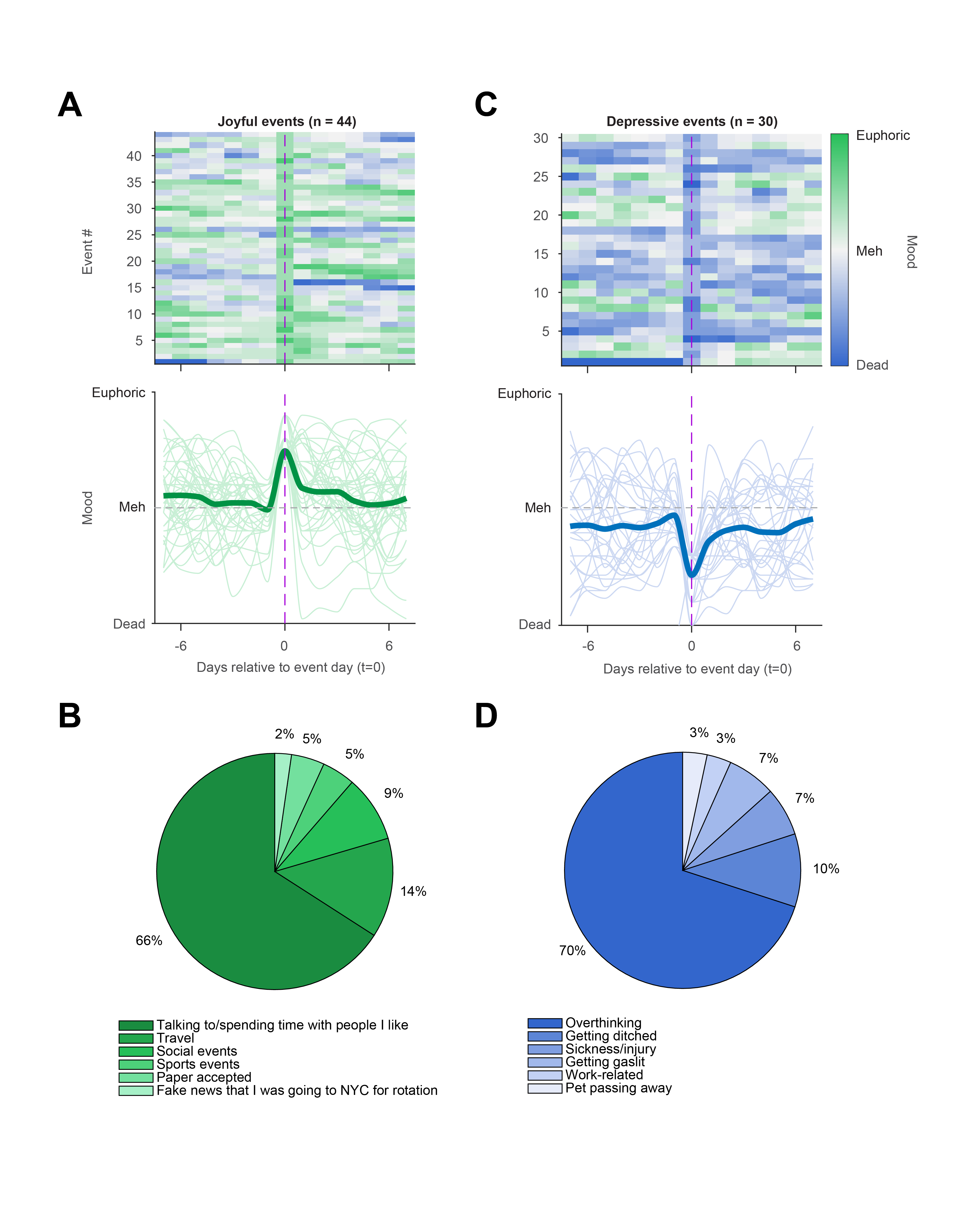
Figure 3. A. Heatmap (top) and individual trajectories (bottom) of mood aligned to joyful events. Each row corresponds to one event; columns indicate days relative to the event day (t = 0). Dashed vertical line marks the event day. Mean trajectories are shown as thick lines; thinner lines represent individual events. B. Proportional breakdown of reported contributors to joyful events. Percentages indicate the fraction of events associated with each category. C. Same as A but for depressive events. D. Same as B but for depressive events.
Additional factors related to mood
Furthermore, I examined several additional factors, some of which were not captured by the event-category summaries above, to assess their relationships with mood. Travel consistently elevated my mood. Mood during travel days was higher than in the preceding days (Fig. 4A left), and it dropped markedly after returning home (Fig. 4A right). Social events were also associated with improved mood (Fig. 4B). However, I did not feel anything special during holidays (Fig. 4C). They were just normal days to me.
I also began therapy in the summer, encouraged by close friends. There was no clear same-day benefit relative to the surrounding week (Fig. 4D). However, across sessions, mood in the week following therapy gradually improved, particularly during the first series (sessions 1–7; Fig. 4E). This pattern could reflect therapeutic benefit, a time-dependent recovery process, or both. I am still in the second series, and by the end of 2025 I had not yet observed comparable improvement yet, unfortunately.
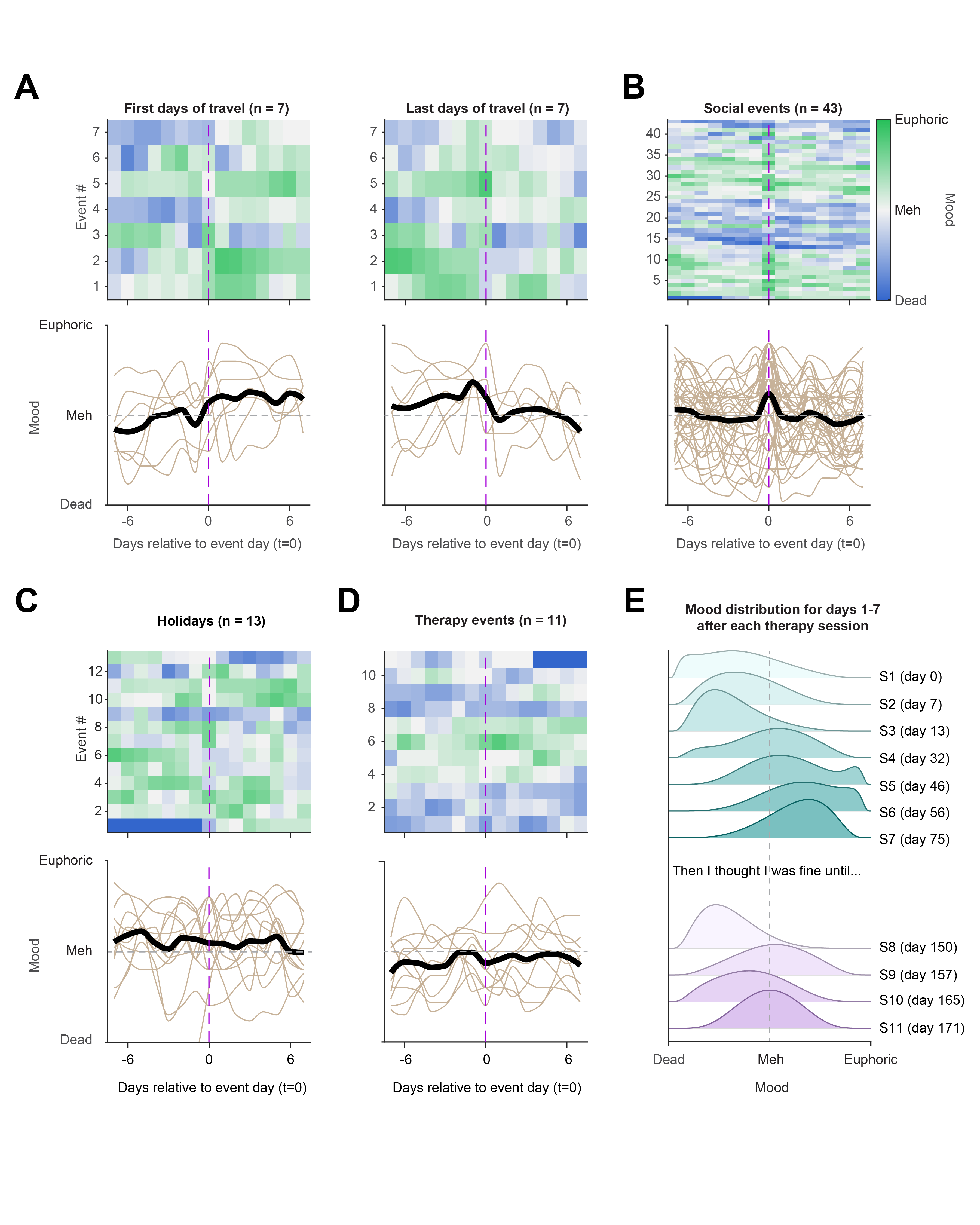
Figure 4. A. Event-aligned mood heatmaps and trajectories for the first and last days of travel and for social events. Plot conventions follow those in Figure 3. B. Same as A but of social events. C. Same as A but of holidays. US holidays: New Year’s Day, MLK day, Memorial Day, Juneteenth, Independence Day, Labor Day, Veterans Day, Thanksgiving, and Christmas Eve. CN holidays: Chinese New Year, Qiming, Dragon Boat Festival, and Mid-Autumn Festival. D. Same as A but of therapy sessions. E. Ridgeline density plots of mood distributions for days 1–7 following each therapy session. Sessions are ordered chronologically from top to bottom.
Relationship between monthly mood and lifestyle variables
Mood can definitely affect health. Some can be causes, while some can be outcomes. Thus, I looked into the relationship between monthly mood and different lifestyle variables, including body weight, daylight exposure, step count, and workout time. It turned out that weight, step count, and workout time showed no meaningful correlations with mood (Fig. 5A, C, D). However, mood showed a moderate positive association with daylight exposure (Fig. 5B), with p = 0.071 which is close to conventional statistical significance threshold. Sunlight helps us produce vitamin D, further supporting mood regulation by influencing serotonin production and reducing inflammation, with deficiencies linked to higher risks of depression, anxiety, and seasonal affective disorder. Guess I will need to sit in the sun for longer time during depression period.
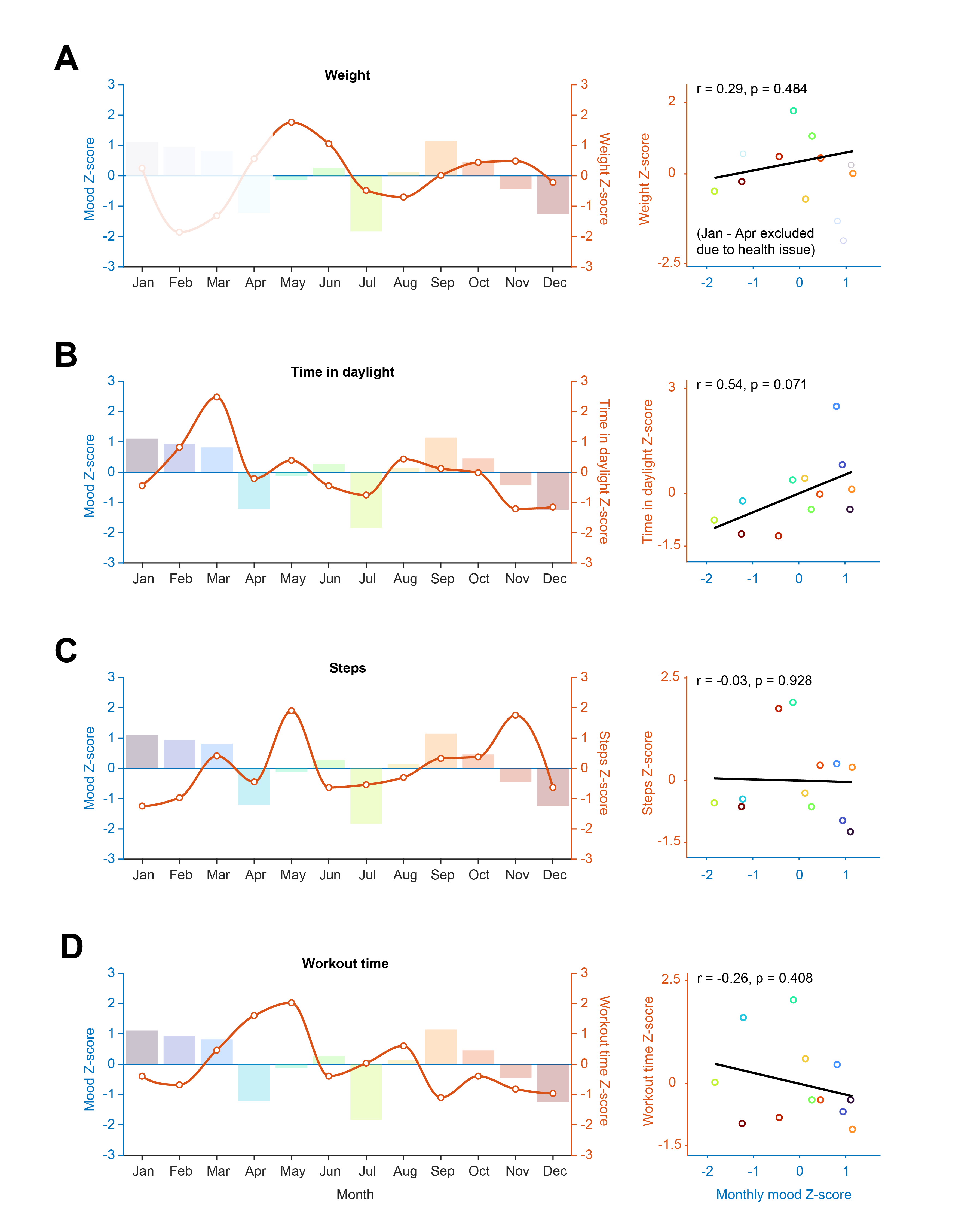
Figure 5. A–D left. Monthly z-scored mood (bars) overlaid with z-scored lifestyle variables (lines), including body weight, time in daylight, step count, and workout time. A–D right. Scatter plots showing correlations between monthly mood z-scores and corresponding lifestyle variables. Each point represents one month and is color-coded by calendar month. Pearson correlation coefficients and two-sided p-values are reported.
Besides vitamin D, music is another powerful regulator of emotional state. As a Swiftie, I always have some go-to albums when I am in different moods. For example, Speak Now, Red, 1989, and Lover accompany periods of emotional stability, whereas Reputation, Folklore, Evermore, and The Tortured Poets Department tend to surface during more difficult times (Fig. 6A).
Not surprisingly, listening time for these two categories showed opposite relationships with mood (Fig. 6B). Dance-around-the-kitchen albums were positively associated with mood (r > 0, p = 0.102, Fig. 6C left), whereas Cry-on-the-cold-hard-ground albums showed a significant negative association (r < 0, p = 0.048, Fig. 6C right).
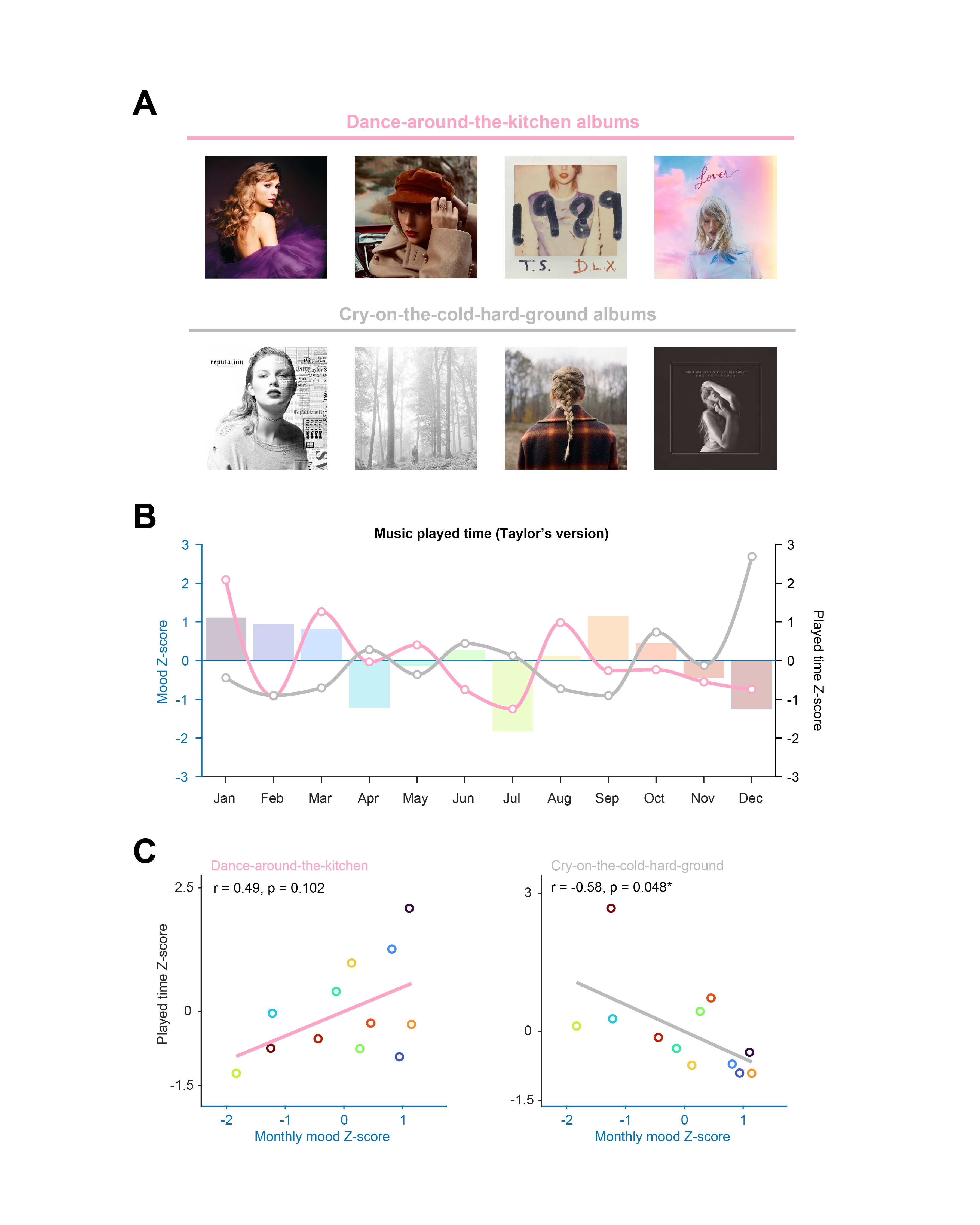
Figure 6. A. Some Taylor Swift albums categorized into two listening modes: “dance-around-the-kitchen” (upbeat/comforting) and “cry-on-the-cold-hard-ground” (sad/ruminative). B. Monthly mood z-scores (colored bars; left axis) overlaid with z-scored music listening time (lines; right axis) for the two listening modes across the year. Points indicate monthly values; curves emphasize month-to-month trends. Colors match month identity across panels. C. Relationship between monthly mood z-score and monthly listening time z-score for each listening mode. Each point represents one month (rainbow colors denote months). Pearson correlation coefficient (r) and two-sided p-value are shown on each panel.
Epilogue
I’m a very nostalgic person who keeps records of nearly everything, including boarding passes, train tickets, movie stubs, postcards, hotel keys, etc. Digitally, I archive calendars, diaries, and health data. However, it is actually the first time that I brought these records together to ask the question whether my life still followed any internal order.
Most of the results matched my expectations since I knew I was happy or down during some certain periods, and I knew what caused it. But for some of the results that I thought there would be a pattern but there was not, like I thought I barely ate during depression so my body weight should be positively correlated to mood, but it did not happen, or still far from statistical significance. It could be using monthly data was not very accurate since not all events happened at the first or last day of the months. I was thinking to use data from every day, but I just don’t have them. Or it just doesn’t work that way of what I thought.
Another challenge was when I was looking back on some specific days to find out why I was joyful or depressed, I had to replay those events in my mind at least one more time. Those memories were so close that like they just happened the day before, but at the same time they were so far away that I know I’d been through a lot since then. For happy events I could still feel the joy, but then realized I don’t and won’t have them anymore. For sad events I could still feel how my heart was broken, and it just kept happening again and again like a cycle. I don’t know when everything could turn any better or even come to an end, or even if they could.
Approaching the end of Evermore, Taylor sings:
“This pain wouldn’t be for evermore.”
That’s very nice of Taylor that she still gave us hope after all the hopelessness. But is it true? Or is it true for me? Guess 2026 will provide the answer. But at least up to today (1/6/2026) it’s like:

Methods
Data acquisition: Mood scores were recorded primarily near the end of each day using Microsoft Excel. In cases of occasional delayed entry, data were logged within three days to minimize recall bias and preserve validity. Lifestyle variables were extracted from Apple Health. Music listening time was obtained from Apple Music monthly Replay reports.
Data visualization: All plots were generated in MATLAB R2024b. Individual observations in box plots were jittered to improve visualization. Final figures were assembled and refined in Adobe Illustrator 2026.
Statistics: Statistical analyses were performed in GraphPad Prism 10 and MATLAB R2024b. For each factor, main effects and interaction terms were evaluated where applicable. Unless otherwise stated, p < 0.05 was considered statistically significant.
Data and code availability
Custom analysis code is available upon reasonable request.
Raw data supporting the current study will be shared upon request. (Actually don’t even think about it. I am not giving you my body weights. 🙂)